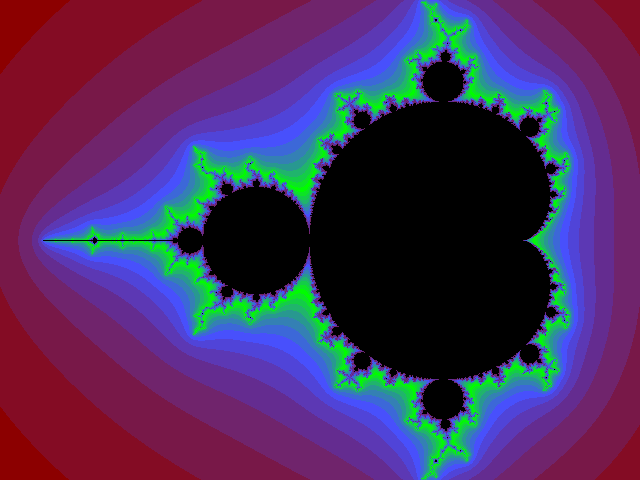
In chaos theory, one often defines sequences of real or complex numbers iteratively: For example, \( z_0=0, z_{n+1}=z_n^2+c \) defines a sequence of complex numbers \(z_0, z_1, z_2,\ldots \) The famous Mandelbrot set corresponds to the set of complex numbers \( c \) for which this sequence is bounded.
This raises an obvious question: can we make sense of terms such as \( z_{1/2} \), i.e., is there a natural and perhaps unique way to iterate a function a non-integer number of times? At age 16, I developed a method to do this, for a large class of functions \( f \) that are to be iterated. For this work, I was awarded a second prize in 1995 at the German youth science competition “Jugend forscht” (more here).
As an entertaining example, consider the Verhulst growth model
\( \large m_0=1,\qquad m_{n+1}=(1+2a)m_n – a m_n^2. \)
A simple transformation shows that this model is equivalent to the logistic map: set \(x_n=a m_n/(1+2a) \), then \( x_{n+1} = r x_n (1-x_n)\), where \( r=1+2a\). Thus, iterating the Verhulst model a non-integer number of times is equivalent to iterating the logistic map a non-integer number of times.
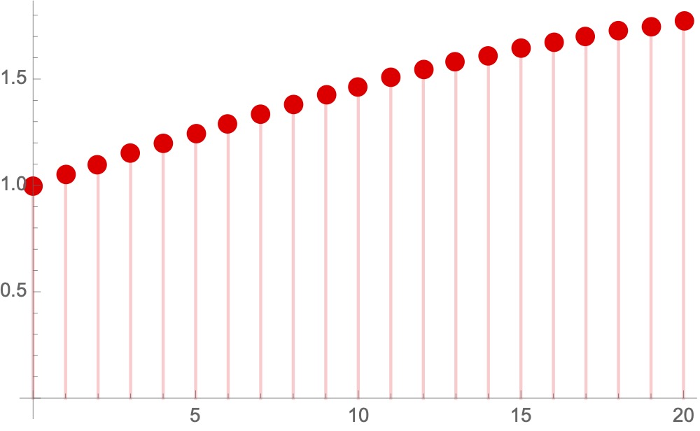
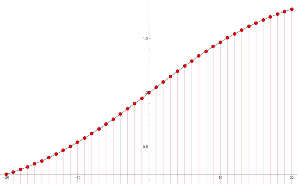
Depending on the constant \( a>0 \), different behaviors of this iterated sequence can be demonstrated. Let us begin with the somewhat “boring” case of \( \mathbf{a=0.05}\). The plot on the left (x-axis: \(n\), y-axis: \(m_n\)) shows the monotonic behavior of the resulting sequence of real numbers.
How, then, should we think of the values “in between” these points? Many ideas for coming up with a natural interpolation method are either arbitrary or based on analogies with, say, the extension of \( a^b \) to non-integer \( b \); however, these analogies turn out not to be applicable in this case.
However, there is a way to do it, resting on two observations. The first observation is that there is a unique natural way to extend the definition of the sequence to negative integer n, which can be done by “iterating backwards”:
\( \displaystyle m_{n-1} = \frac{1+2a-\sqrt{1+4a(1+a-m_n)}}{2a}.\)
This allows us to determine \(m_{-1}\), \(m_{-2}\), and so forth.
The second observation is that \( m_n \) behaves very regularly as \( n\) tends to minus infinity: the fraction \( m_n/m_{n-1} \) is almost constant on large intervals of \( n\). Consequently,
\( \displaystyle m_{n+c}\approx m_n\cdot \left(\frac{m_{n+1}}{m_n}\right)^c\qquad \mbox{as }n\to -\infty.\)
If this is true for integer \( c \), it should also be true for non-integer \( c \), and this allows us to approximate, for example, the values of \( m_{n+\frac 1 2} \) for negative integer \( n \), expecting that this approximation gets better in some sense as \( n \) tends to minus infinity. But once we have the approximate value of, say, \( m_{-100.5} \), we can iterate our way forward to \(m_{-99.5}\), \( m_{-98.5}\) and so on, assuming that the defining iteration law above is still valid, and arrive at \( m_{0.5}\). We can then define this value as what we obtain from this process in the limit of \( n \) tending to minus infinity.
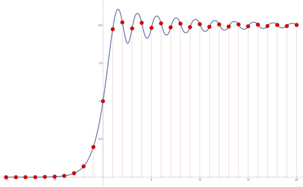
What we get looks like a very natural interpolation indeed, and it is guaranteed to satisfy the recursion law above, see Plot 2. Values for integer arguments are shown as the red dots.
Note that we have not formally proven that this limit procedure converges. It would be nice to demonstrate this, and to show that the resulting function is smooth (or analytic – this prescription admits also complex numbers of iterations).
It should also be possible to show that this interpolation is the unique function that satisfies the recursion law and that behaves regularly in some particular sense at minus infinity (say, its logarithm is approximately linear, or concave, at small enough arguments). This might be similar to the well-known uniqueness statements on the interpolation of the factorial by the Gamma function.
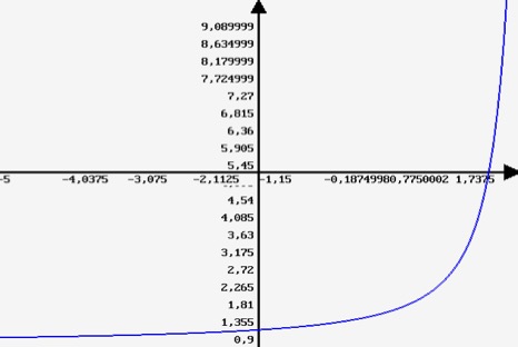
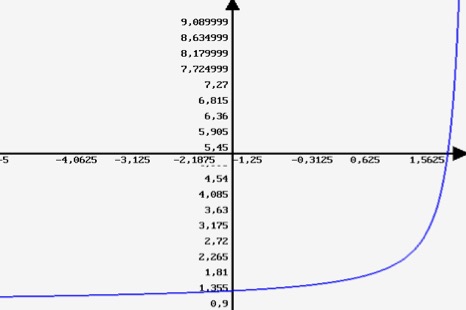
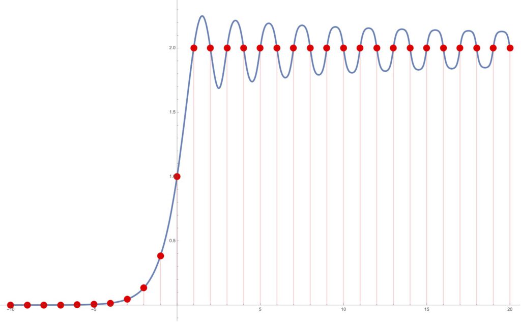
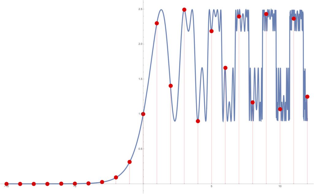
The results of this method become much more interesting for larger values of \( a ). Chaotic behavior is known to occur at integer values of iterations, but what does it look like at non-integer arguments? The plots below show that the behavior is quite interesting and surprising indeed.

Higher-order operations: pentation and hexation at non-integer arguments
The idea of higher-order operations is described in this Wikipedia article (see also the references therein) – however, standard treatments overlook the fact that the number of different operations doubles at each level, as we will see. First, note that multiplication can be understood as repeated addition, and exponentiation is repeated multiplication:
\( \large a\cdot b = \underbrace{a+a+\ldots +a}_b,\qquad a^b=a\hat{ }b=\underbrace{a\cdot a \cdot \ldots \cdot a}_b. \)
This suggests that we continue the construction, and define a new operation in terms of “power towers” that has been termed tetration. There are, however, two natural options for how to do this:
\( \large a\uparrow b = \underbrace{a\hat{ } ( a\hat{ } ( \ldots \hat{ }(a\hat{ } a )))}_b,\qquad a\downarrow b = \underbrace{(((a\hat{ } a)\hat{ } a)\hat{ } a\ldots}_b .\)
Typically, the first option is used as the definition, and the second option is dismissed, because of the simple closed-form expression \(a\downarrow b=a^{a^{b-1}}\). But I believe this is a mistake: after all, if we go to even higher-order operations (pentation, hexation, …), the number of operations will double, but both options will be non-trivial. Therefore, there are four different pentation operations \( a \uparrow \uparrow b\), \(a \uparrow\downarrow b\), \( a\downarrow\uparrow b\), \(a\downarrow\downarrow b\). They are characterized by four different recursion relations
\( \large \begin{eqnarray*} a\uparrow\uparrow (b+1) &=& a\uparrow (a\uparrow\uparrow b),\\ a\uparrow\downarrow (b+1) &=& a\downarrow (a\uparrow\downarrow b),\\ a\downarrow\uparrow(b+1)&=&(a\downarrow\uparrow b)\uparrow a,\\ a\downarrow\downarrow (b+1)&=&(a\downarrow\downarrow b)\downarrow a. \end{eqnarray*}\)
One of the questions that arise naturally is how the case of non-integer \( b\) can be treated. In the case of exponentiation, the idea of “repeated multiplication” will not tell you what \( a^{\frac 1 2}\) is, but there are laws such as \( a^m a^n = a^{m+n} \} which immediately allow you to find the unique definition that makes sense. However, for tetration and higher-order operations, no such laws are available.
In my “Jugend forscht” work, I have applied the idea described above (see the Verhulst process interpolation) to this question. It turns out that this idea, unfortunately, does not work for (the non-trivial version of) tetration. However, it seems to work, for example, for the binary pentation function
\( \large \mathfrak{P}(x)=2\downarrow\uparrow x = 2\downarrow\downarrow x. \)
This function is characterized by the recursion relation
\( \large \mathfrak{P}(1)=2,\qquad \mathfrak{P}(x+1)=\mathfrak{P}(x)^{\mathfrak{P}(x)}.\)
This very old PDF document describes how it can be done, and gives several further observations. An evaluation of non-integer exponents is also possible for the binary hexation function
\( \large \mathfrak{H}_2(x)=2\downarrow\downarrow\downarrow x.\)
The numerical results are shown in the graphs below. Apologies for the bad graph quality from my old Amiga 500 teenage days. The plots indicate that the method of interpolation is indeed a natural one that seems to lead to smooth (and potentially analytic) functions.